Designing Data Intensive Applications Notes: Ch.3 Storage and Retrieval
aboelkassem | November 02, 2023
Continuing our series for “Designing Data-Intensive Applications” book.
In this article, we will walkthrough the second chapter of this book Chapter.3 Storage and Retrieval.
Table of content
Data Structures That Power Your Database
Imagine having the world’s simplest database at your disposal, implemented using just two Bash functions. This minimalist yet functional database allows you to store and retrieve key-value pairs effortlessly. Here’s the code snippet that brings this database to life:
#!/bin/bash
db_set () {
    echo "$1,$2" >> database
}
db_get () {
    grep "^$1," database | sed -e "s/^$1,//" | tail -n 1
}
This two functions: Append only writes and For lookups read O(n)
An index is an additional structure that is derived from the primary data (metadata)
Log Structured Storage (Hash Index)
Whenever you append a new key-value pair to the file, you also update the hash map to reflect the offset of the data you just wrote

Append only Data structure. The log file is sequentially written, which allows for fast write operations since it avoids random disk seeks.
What if the disk is full or out of space? we will group the logs into segments with size
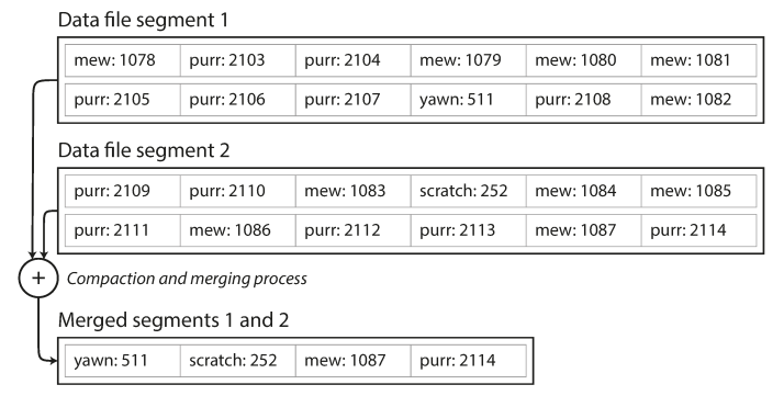
New records are appended to a segment of certain size which is being merged and compacted by a background thread.
While it is going on, we continue read and write using the old segment files until the merging process is complete, we switch read requests to using the new merged segment instead of the old segments and finally the old segments are deleted.
The issues of this index and how to solve them
- File format: CSV is not the best format for a log, It’s faster and simpler to use a binary format
- Deleting records: Use special deletion record called tombstone, just mark this data with deleted flag and the merging process to discard it.
- Crash recovery: If the database is restarted, the in-memory hash maps are lost, so we save a snapshot of each segment’s hash map on disk.
- Concurrency control: Use one thread for writing and multiple threads for reading
- Partially written records: to prevent corrupted data, we add checksum
The Props of Log structured hash index
- Sequential write operations is faster than than random writes
- Concurrency and crash recovery are much simpler, the system can replay the log file to restore the database to a consistent state.
- No data fragmentation (meaning the data is stored distributed on the hard disk)
The limitations of Log structured hash index
- The hash table must fit in memory (for fast read/writes), so you have a space issue
- Range queries are not efficient
SSTable (Stored String Tables)
To Fix the memory space issue, we will use this SSTable
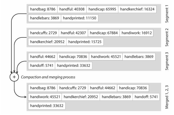
This work by sorting the keys, which will make the keys unique after merge process
- Each key will appear once in the segment
- Each segment will be sorted by key
- Keep separate hashtable for each segment
-
Merge each segments into one segment like the following
- you start reading the input files side by side, look at the first key in each file, copy the lowest key (sorted) to new merged segment and repeat.
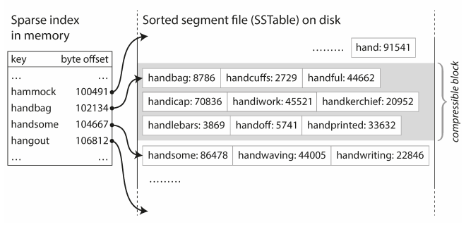
Then, The hash map index will contains the first key of each segment instead of all keys
- Each segment will be sorted by key
- Keep separate hashtable for each segment
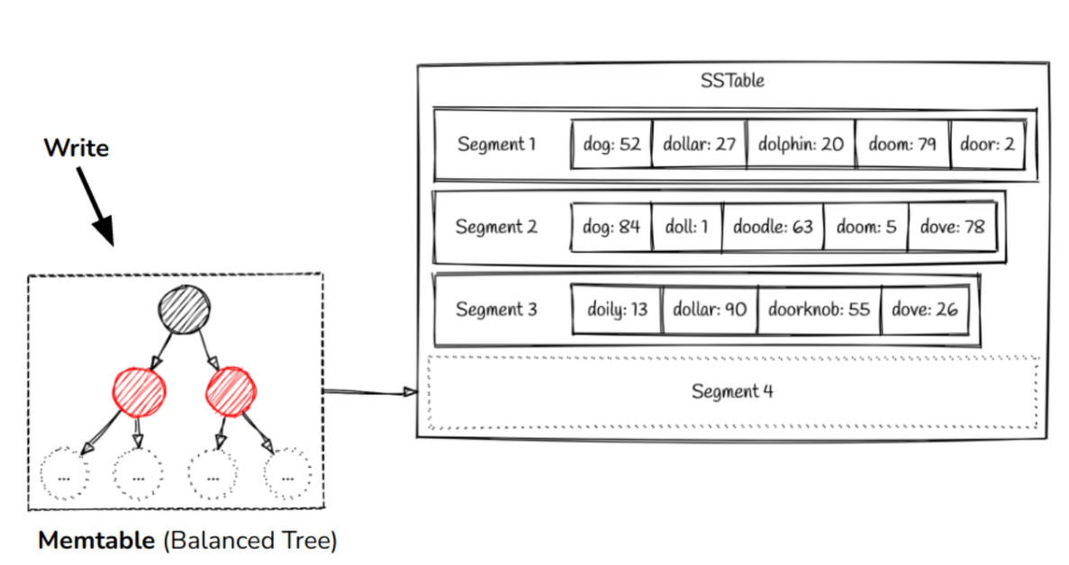
How to save the segments sorted on memory, Our incoming writes can occur in any order? We will use AVL Tree.
The flow to save data
- When a write comes in, add it to an in-memory balanced tree data structure called memtable
- When the memtable gets bigger than some threshold (for example > 100 MB), write it out to disk as an SSTable file (Segment) which is the most recent segment
- In order to serve a read request, first try to find the key in the memtable, then in the most recent on-disk segment, then in the next-older segment, etc
- From time to time, run a merging and compaction process in the background to combine segment files and to discard overwritten or deleted values
This algorithm (named also LSM Tree) used in LevelDB, RockDB, Cassandra, HBase and Lucene engine (used in Elastic Search and Solr) LSM-Trees offer an efficient segment merging mechanism, eliminate the need for an in-memory index for all keys, and support grouping and compressing records before writing to disk, but they can be slow for non-existent key lookups (which can be improved with a bloom filter).
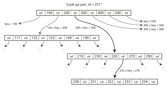
B-Tree
This is the most widely used indexing in Relational Databases like Postgres. Like SSTables, B-trees keep key-value pairs sorted by key which allows efficient keyvalue lookups and range queries.
Unlike SSTable (which break the database into segments), B-Tree break the database into fixed Size blocks (pages). Each page is have size (traditionally 4 KB in size)
Unlike SSTable (which is stored on memory), B-Tree is in the disk
B-Tree is balanced, so n keys always have depth of O(log n). It also have a branching factor of several hundreds typically.
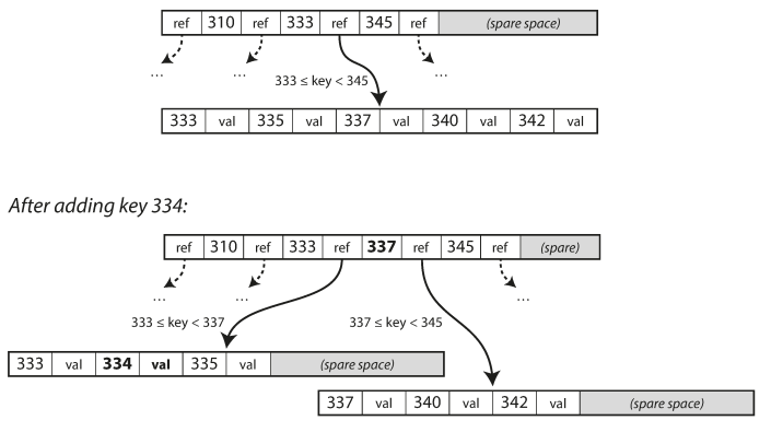
If you want to update the value for an existing key in a B-tree, you search for the leaf page containing that key, change the value in that page, and write the page back to disk.
If you want to add a new key, you need to find the page whose range encompasses the new key and add it to that page.
- If there isn’t enough free space in the page to accommodate the new key, it is split into two half-full pages, and the parent page is updated to account for the new subdivision of key ranges
Most databases can fit into a B-tree that is three or four levels deep, so you don’t need to follow many page references to find the page you are looking for. (A four-level tree of 4 KB pages with a branching factor of 500 can store up to 256 TB.)
B-Tree Reliability
In order to make the database resilient to crashes
- B Tree uses Write Ahead Log (WAL) ⇒ This is an append-only file to which every B-tree modification must be written before it can be applied to the pages of the tree itself.
To Improve the previous way for performance,
- They use a new way called Copy On Write scheme, Any new data is written to a different location, and a new version of the parent pages in the tree is created, pointing at the new location.
- Another optimization way is to use short key names (B-Tree+)
- Another optimization way is to use Extra pointers for each node to point previous and next nodes
B-Tree vs SSTable
Other Indexes
Secondary Index
This index based on secondary key (foreign key) when doing joins between table for better performance. The main difference between primary key and foreign that keys are not unique. Both B-Trees and LSM-Trees can have secondary indexes.
It stores the reference (pointer) of the location in the head file (the place where actual rows are stored).
When updating a new value:
- If the new value is not larger than the old value, it will just override and keep the same reference (key) which will be good for writes performance
- Else, We will need to provide extra space on the disk and this will require new reference key in the heap (all indexes need to be updated to point at the new heap location)
The last point will reduce the performance for reads (because the heap location has changed to another location in the disk).
Clustered Index
To solve previous mentioned issue, we will store the actual row within the index (called clustered index).
Once I reached to the key, it will contains the data as well.
In SQL Server, primary index is always clustered index and you can specify one clustered index per table.
There is another index called covering index which stores some of a table’s columns within the index (not all data).
Efficient for reads but they require additional storage and can add overhead on writes.
Multi Column Index
Called also (Composite Index) which combines several fields into one key by appending one column to another.
The order of fields is very matter (because there is a relation and depends on it) like old phone book search, which provide an index from (lastName, firstName) to phone number.
- Due to the sort order, the index can be used to find all the people with a particular last name, or all the people with a particular (lastName, firstName) combination. However, the index is useless if you want to find all the people with a particular first name.
An example of this index is a geospatial index which is used to search by latitude followed by longitude.
SELECT * FROM restaurants
WHERE latitude > 51.4946 AND latitude < 51.5079
AND longitude > -0.1162 AND longitude < -0.1004;
Since in this case, the order is matter and latitude related to longitude, A standard B-tree or LSM-tree index is not able to answer that kind of query efficiently: it can give you either all the restaurants in a range of latitudes.
Other use cases
- On an e-commerce website you could use a three-dimensional (combination) index on the dimensions (red, green, blue) to search for products in a certain range of colors
- Weather observations you could have a two-dimensional index on (date, temperature) in order to efficiently search for all the observations during the year 2013 where the temperature was between 25 and 30℃.
Full-Text Search and Fuzzy Index
This index allows you to query for similar keys such as misspelled words.
This index does normalization, lemmatization, and stemming for each word. which ignores grammatical variations of words, and searches for occurrences of words near each other in the same document, and support various other features that depend on the linguistic analysis of the text.
Lucene engine (used in elastic search) uses an SSTable-like structure (small in-memory index) that tells queries at which offset in the sorted file they need to look for a key.
Storing Data In-Memory
In-memory databases are much faster but less durable and more expensive.
Memcached is caching DB where it’s acceptable for data to be lost if a machine is restarted.
To make sure of durability, writing a log of changes to disk with periodic snapshots, or by replicating state to other machines. When an in-memory database is restarted, it needs to reload its state, either from disk or over the network from a replica.
Products such as VoltDB, MemSQL, and Oracle TimesTen (Not free) are in-memory databases with a relational model, and the vendors claim that they can offer big performance improvements by removing all the overheads associated with managing on-disk data structures.
Redis and Couchbase (open source) provide weak durability by writing to disk asynchronously.
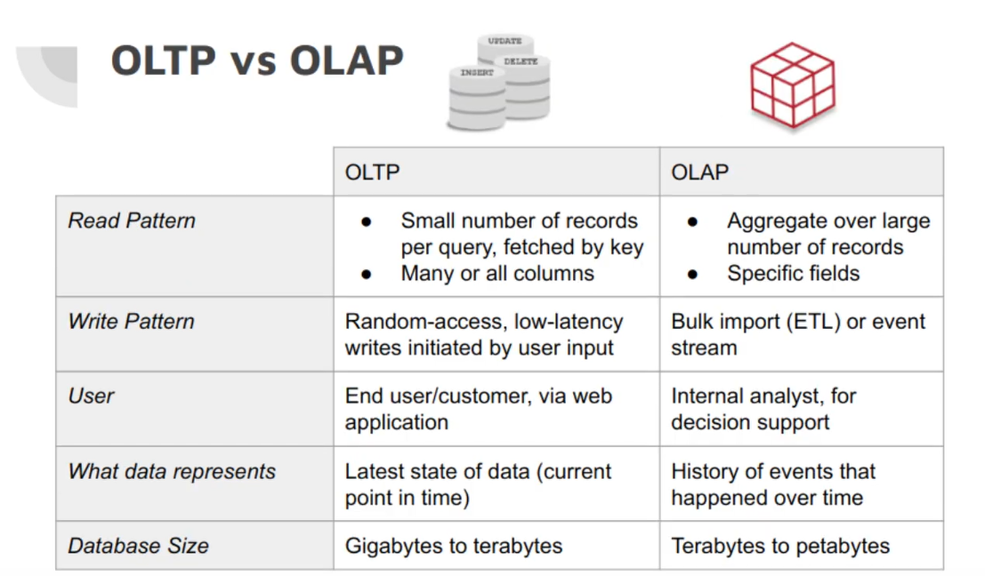
Online Transaction Processing (OLTP) vs Analytics Processing (OLAP)
Online Transaction Processing (ALTP) is a pattern to read some specific rows/data in the database (a transaction to DB)
- A transaction needn’t necessarily have ACID (atomicity, consistency, isolation, and durability) properties. Transaction processing just means allowing clients to make low-latency reads and writes as opposed to batch processing jobs (analytics OLAP), which only run periodically(for example, once per day).
- Supported databases: MySQL, Oracle, PostgresSQL, Cassandra, SAP HANA, SQL Server
Online Analytics Processing (ALTP) is used for data analysis which perform analytic query needs to scan over a huge number of records, only reading a few columns per record, and calculates aggregate statistics (such as count, sum, or average) rather than returning the raw data to the user.
- Supported databases: Spark, Apache Hive, Teradata, RedShift, Cloudera, Impala, Presto, Drill, Cassandra SAP HANA, SQL Server
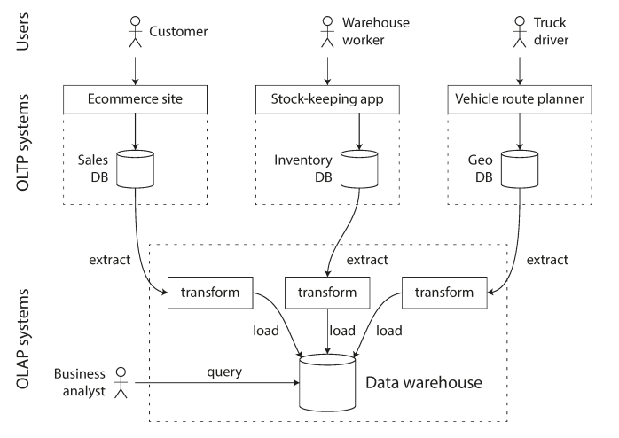
At first, you can use the same database with these two patterns OLTP and OLAP like SQL Server, but early 1990s, there was a trend for companies to stop using their OLTP systems for analytics purposes. This database called Database warehouse.
Database Warehouse
A separate Database to perform huge OLAP queries.
The data warehouse contains a read-only copy of the data in all the various OLTP systems in the company.
Data is extracted from OLTP databases (using either a periodic data dump or a continuous stream of updates), transformed into an analysis-friendly schema, cleaned up, and then loaded into the data warehouse. This process of getting data into the warehouse is known as Extract–Transform–Load (ETL).
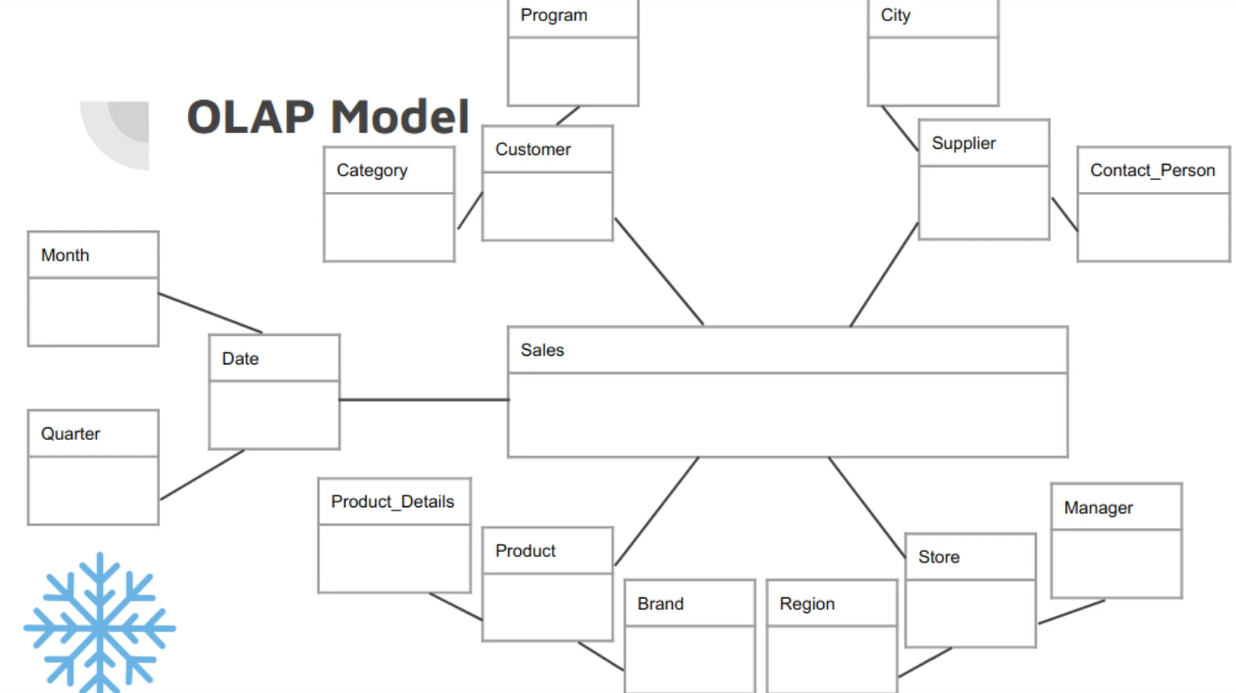
Stars and Snowflakes: Schemas for Analytics
These two schemes are used for data warehouse and OLAP
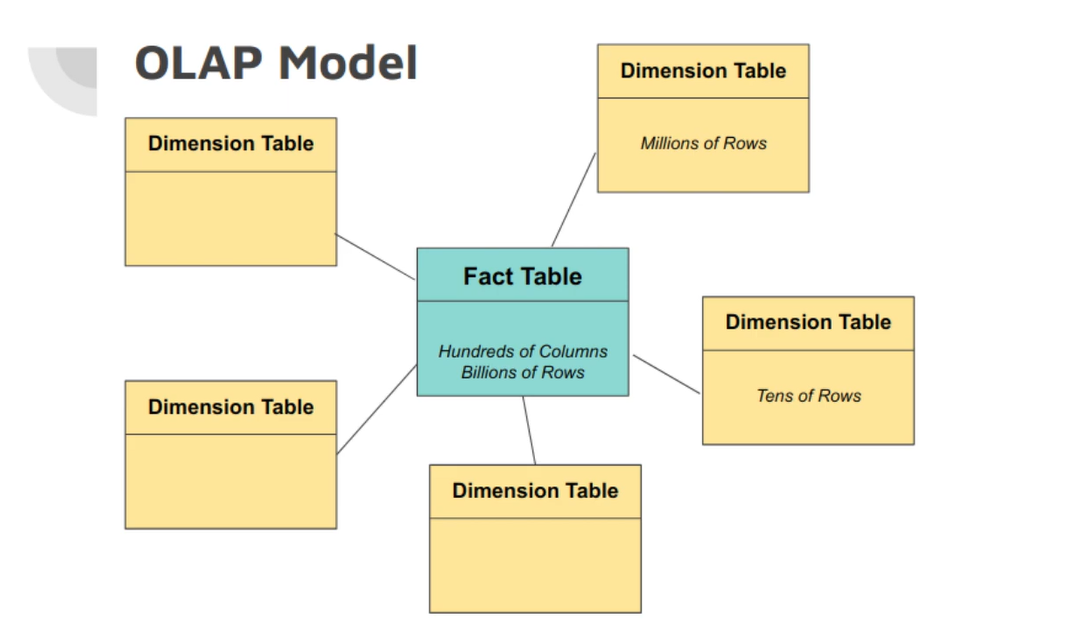
Star Scheme
The main and big table called fact table while other tables called Dimension table The fact table determined based on business, it can be Transaction table for banking, sales table .. etc
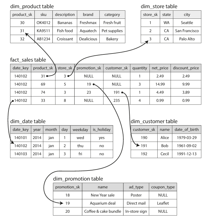
Snowflakes Scheme is like Star scheme but more normalized
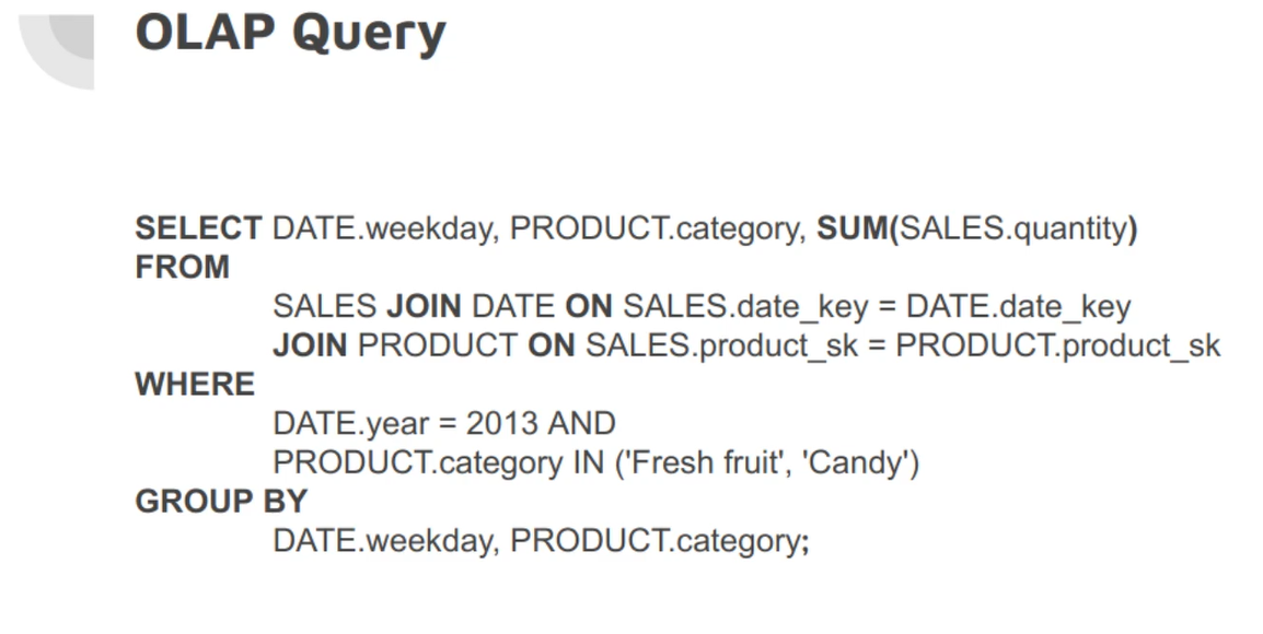
Example of OLAP query to know whether people are more inclined to buy fresh fruit or candy, depending on the day of the week.
Comparison of OLTP vs OLAP
Column Storage
For OLAP, if your fact table have trillions of rows and hundreds of columns and want to doing a query to only access 4 or 5 columns like the following query
SELECT
	dim_date.weekday, dim_product.category,
	SUM(fact_sales.quantity) AS quantity_sold
FROM fact_sales
	JOIN dim_date ON fact_sales.date_key = dim_date.date_key
	JOIN dim_product ON fact_sales.product_sk = dim_product.product_sk
WHERE
	dim_date.year = 2013 AND
	dim_product.category IN ('Fresh fruit', 'Candy')
GROUP BY
	dim_date.weekday, dim_product.category;
In most of OLTP databases, the storage is row-oriented fashion (rows are stored next to each other in the disk), which the storage engine still needs to load all rows of all columns from disk into memory to parse them and filter out those that don’t meet the required conditions. What can take a long time.
So, the column-oriented storage will be more suitable for that case. Which instead of storing all values of rows together, we will store all values of columns together instead.
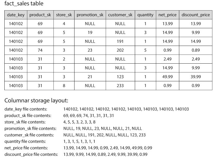
We will store each column into a file containing the value rows.
The benefits of Columnar storage
- Efficient performance for reads and aggregations on specific columns
-
Compression Support with Bitmap and Run-length encoding for product_sk column example.
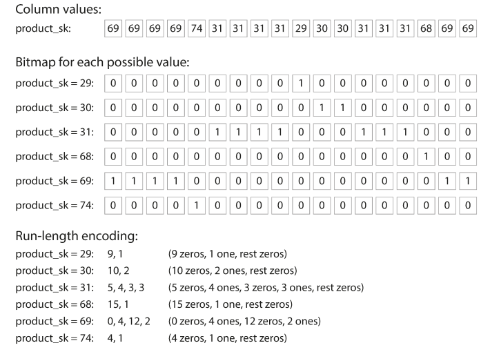
Bitmap helps with reads query like WHERE IN (like WHERE product_sk IN (30, 68, 69)), WHERE AND (like WHERE productsk = 31 AND storesk = 3) which apply AND, OR operators to binary indexes.
-
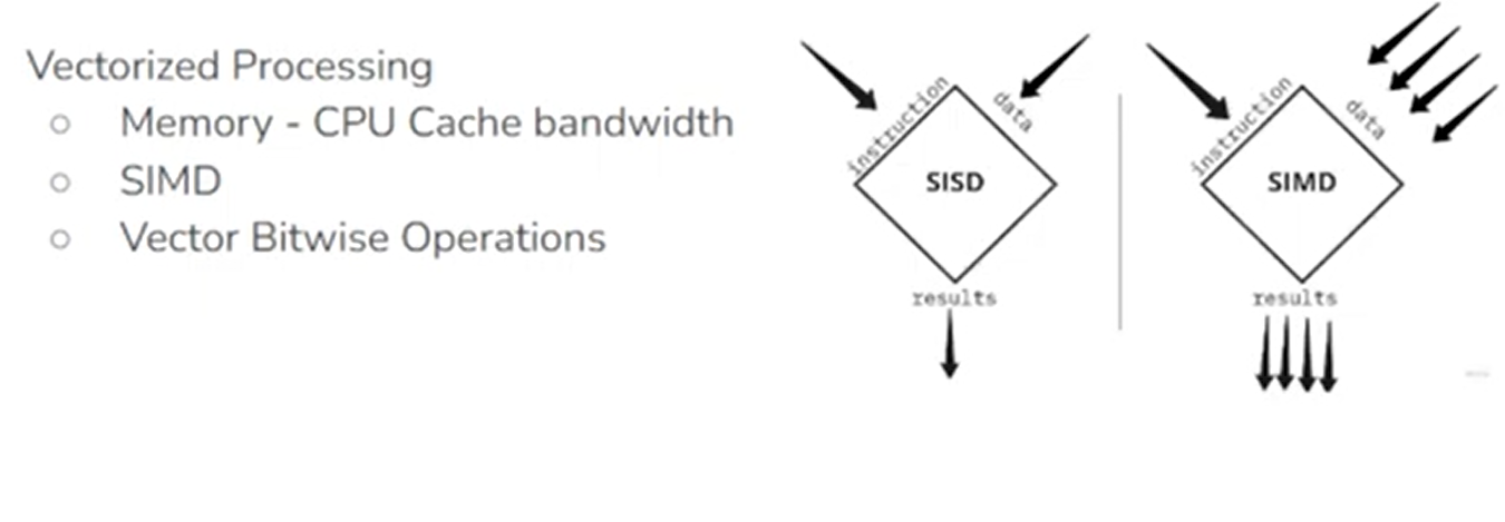
Vectorized processing with SIMD (single instruction multiple data)
- For Sorting, We don’t sort single column and leave the others unchanged.
A helpful technique for data warehouse is materialized aggregates, which caches some of the aggregated data that are used most often. In the relational model, this can be created using materialized views.